quantitray

An R package to calculate MPN (most probable number) from IDEXX Quanti-Tray, Quanti-Tray/2000, and Quanti-Tray/Legiolert tests.

Installation

devtools::install_github("jknappe/quantitray")

Load the package

library(quantitray)

Quanti-Tray tests

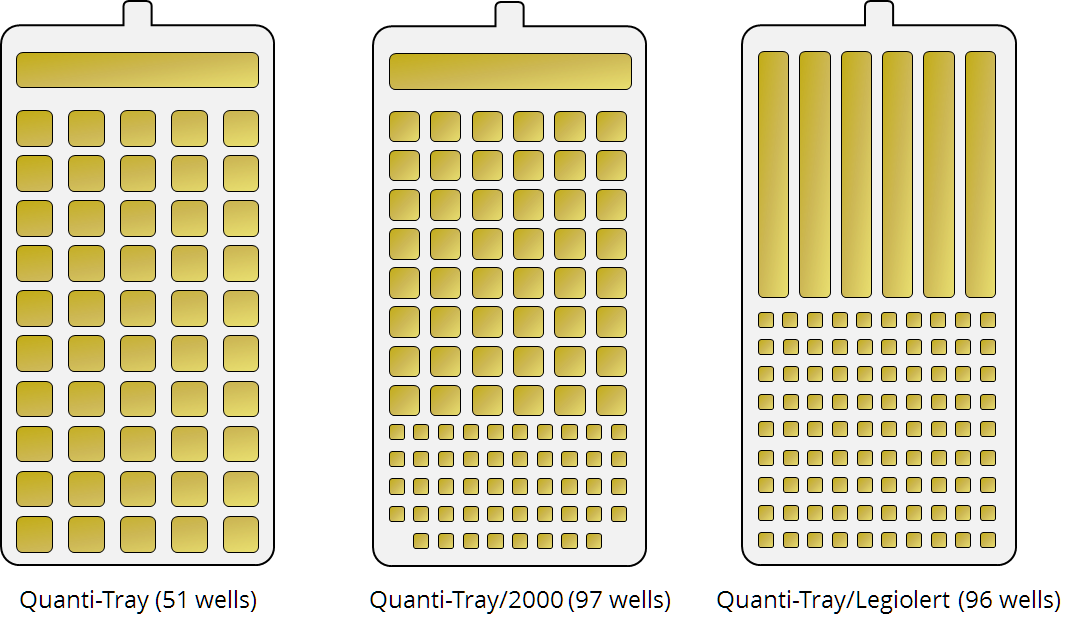
Quanti-Tray tests allow to quantify bacterial counts in water samples. IDEXX Technologies offer three types of Quanti-Tray trays: Quanti-Tray (with 51 large wells), Quanti-Tray/2000 (with 49 large trays and 48 small trays), and Quanti-Tray/Legiolert (with 6 large trays and 90 small wells).

Quantitrays

For detailed description on how to use the tests and interprete the test results, please refer to the documentation provided by the manufacturer here: https://www.idexx.com/en/water/water-products-services/quanti-tray-system/

Quanti-Tray and Quanti-Tray/2000 are used for quantifying coliforms, E. coli, enterococci, Pseudomonas aeruginosa, and Heterotrophic Plate Counts (HPC).Quanti-Tray/Legiolert is used for quantifying Legionella pneumophila.

Converting well counts to bacterial counts

Solutions provided by the manufacturer

The manufacturer provides printable lookup tables on its website to convert from well counts to bacterial counts.

The manufacturer also provides a ‘Windows’-based software solution for download on its website to convert from well counts to bacterial counts.

Solutions provided in this package

This package offers a set of functions to convert well counts to bacterial counts in R using the lookup tables provided by the manufacturer.

Conversion functions

This package introduces conversion functions from well counts to bacterial counts:

quantify_mpn(large, small, method) to convert well counts to numeric point estimate MPN (in MPN/100 ml)
quantify_95lo(large, small, method) to convert well counts to numeric lower 95% confidence interval MPN (in MPN/100 ml)
quantify_95hi(large, small, method) to convert well counts to numeric upper 95% confidence interval MPN (in MPN/100 ml)

Arguments

large needs to be a positive integer representing the number of positive large wells counted (mandatory for all methods)
small needs to be a positive integer representing the number of positive small wells counted (mandatory for methods “qt-2000” and “qt-legio)
method specifies the Quanti-Tray method used: “qt” for Quanti-Tray, “qt-2000” for Quanti-Tray/2000, “qt-legio” for Quanti-Tray/Legiolert (mandatory)

Edge cases

To provide coherent function output (numeric values or a list of numeric values), values above and below the method detection limit are handled as follows:

For results below the detection limit (no positive wells), the quare root of the method detection limit is returned as point estimate.
For results above the method detection limit (all positive wells), only the lower confidence interval is returned as numeric value, whereas point estimate and upper confidence interval are returned as NA.

Lookup tables

The lookup tables provided by the manufacturer can be accessed in R after the package is loaded. This might be useful to implement reverse lookups.

quanti_51 provides data for the QuantiTray (including MPN point estimate and 95% confidence intervals)
quanti_96 provides data for the QuantiTray/Legiolert (only MPN point estimate; confidence intervals are not provided)
quanti_97 provides data for the QuantiTray/2000 (including MPN point estimate and 95% confidence intervals)

Examples

Single conversions to point estimate

The conversion functions can be used to convert a single result. Note, that when using the Quanti-Tray test with 51 wells (argument method = "qt"), only large wells (argument large) need to be defined.

library(quantitray)

# Quanti-Tray test with 51 wells
quantify_mpn(large = 42, method = "qt")
## [1] 88.5

# Quanti-Tray/2000 test with 97 wells
quantify_mpn(large = 42, small = 23, method = "qt-2000")
## [1] 156.13

# Quanti-Tray/Legiolert test with 96 wells
quantify_mpn(large = 5, small = 23, method = "qt-legio")
## [1] 78.8

Single conversions to confidence intervals

Note, that when using the Quanti-Tray/Legiolert test with 96 wells (argument method = "qt-legio"), confidence intervals cannot be calculated (as the lookup tables provided by the manufacturer only include information for the point estimate).

library(quantitray)

# Quanti-Tray test with 51 wells
quantify_95lo(large = 42, method = "qt")
## [1] 63.9

# Quanti-Tray test with 51 wells
quantify_95hi(large = 42, method = "qt")
## [1] 126.2

# Quanti-Tray/2000 test with 97 wells
quantify_95lo(large = 42, small = 23, method = "qt-2000")
## [1] 120.45

# Quanti-Tray/2000 test with 97 wells
quantify_95hi(large = 42, small = 23, method = "qt-2000")
## [1] 200.41

Vectorial conversions and pipes

All conversions are vectorized and can be used within pipes.

library(quantitray)
library(tidyverse)

counts_qt2000 <- 
  tibble(l_well = seq(0, 4, 1), s_well = seq(0, 8, 2))
  
results_qt2000 <-
  counts_qt2000 %>%
  mutate(qt_95lo = quantify_95lo(l_well, s_well, "qt-2000"),
         qt_mpn  = quantify_mpn(l_well, s_well, "qt-2000"),
         qt_95hi = quantify_95hi(l_well, s_well, "qt-2000"))

results_qt2000

## # A tibble: 5 x 5
##   l_well s_well qt_95lo qt_mpn qt_95hi
##    <dbl>  <dbl>   <dbl>  <dbl>   <dbl>
## 1      0      0    0      0       3.67
## 2      1      2    0.62   3.01    7.33
## 3      2      4    2.32   6.09   12.1 
## 4      3      6    4.42   9.24   16.9 
## 5      4      8    6.94  12.5    20.5 